Contents
- Introduction to DAG
- Quantify potential associations or bias for given DAG
- Introduction
- Download Stata commands
- Steps for a single simulation and quantification
- Example 1: a classical triangle
- Example 2: an intermediate variable
- Example 3: Collider stratification bias
- Example 4: M structure or M bias
- Reference
- A list of examples of DAG applied to researches
Introduction to DAG
Under development
Quantify potential associations or bias for given DAG
Introduction
We know that one of the drawbacks in the use of DAGs is that DAGs show the causal relationships among variables in a qualitative manner. However, in some cases, we actually may want to quantify the causal relationships. This drawback may to some extent be overcome by using simulation methods.
Download Stata commands
We have developed two Stata commands (ancestor, child) to carry out the simulation and quantification. Type and run "ssc describe dag" in the Stata command window. You should be able to view and download the commands.
The package has been updated in the 22nd August 2019, previous version simulate only binary variables and the current can simulate normally distributed continous variables as well. Please re-install the package if you had a previous version. The downloaded commands are located under two folders: ado/plus/c and ado/plus/d
We are working on A stata command drawing a high quanlity DAG.
Steps for a single simulation and quantification
- Identify ancestor-variables and child-variables
- Simulate a dataset with all ancestor-variables
- Generate the child-variables
- Quantify the associations
Example 1: a classical triangle

-
Interpretation of the DAG:
Under development
-
Curious questions:
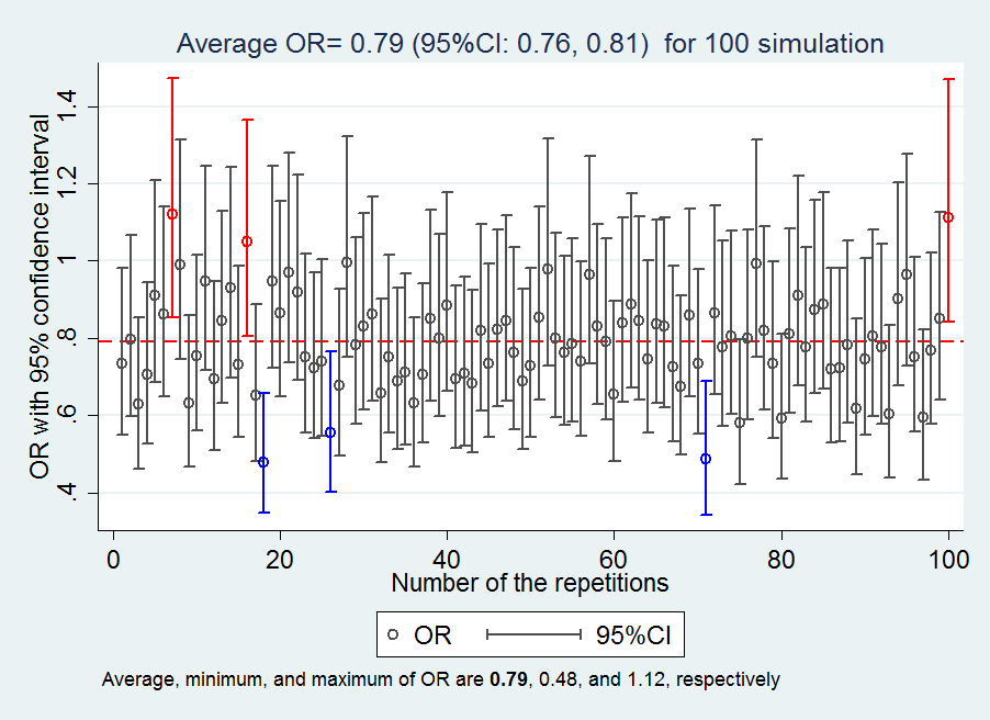
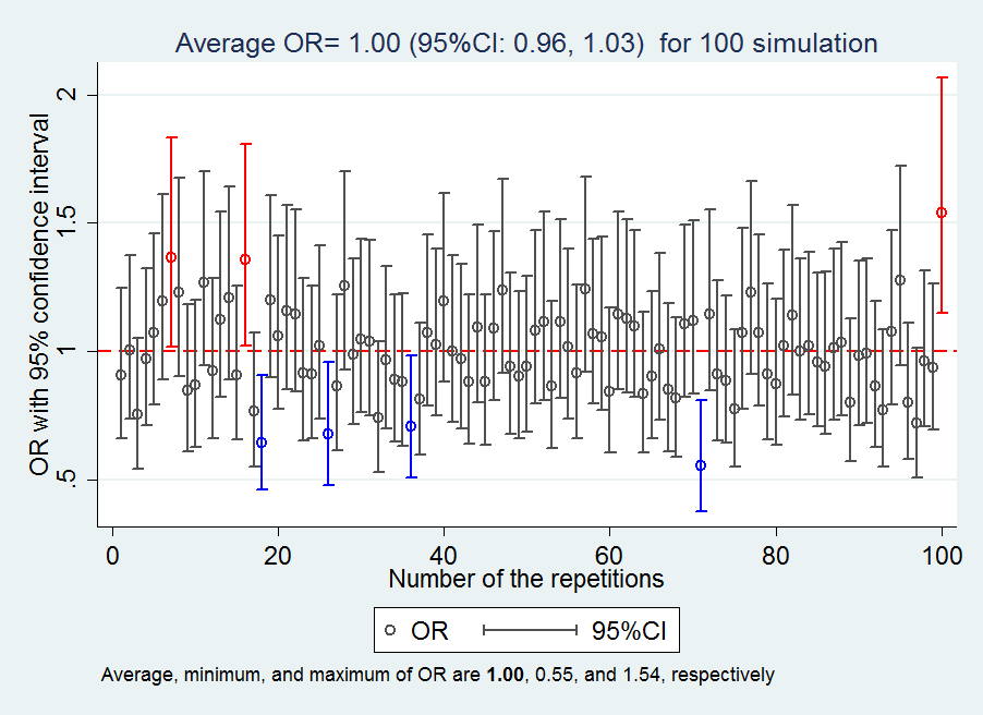
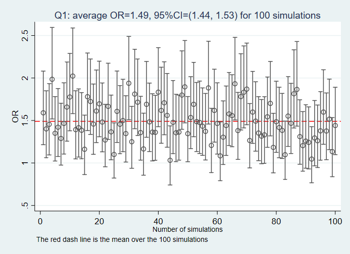
Q1: Given the DAG, what the association between the variable E and D would be if the variable C is not adjusted for?
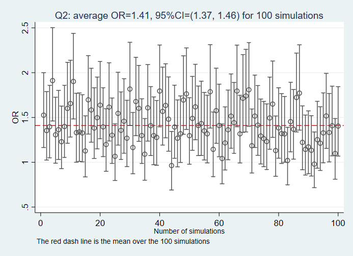
Q2: Given the DAG, what the association between the variable E and D would be if the variable C is adjusted for?
-
Simulation and quantification:
Single Simulation and quantification
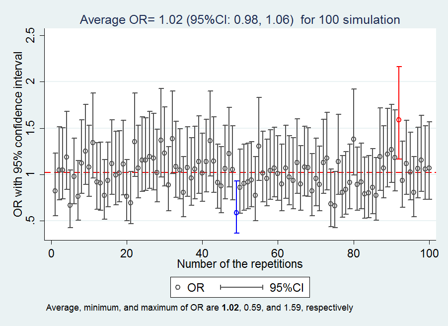
Multiple Simulations and quantification
-
Answers to the questions:
Example 2: an intermediate variable

-
Interpretation of the DAG:
Under development
-
Curious questions:
Q1: Given the DAG, what the association between the variable E and D would be if the variable I is not adjusted for?
Q2: Given the DAG, what the association between the variable E and D would be if the variable I is adjusted for?
-
Simulation and quantification:
Single Simulation and quantification
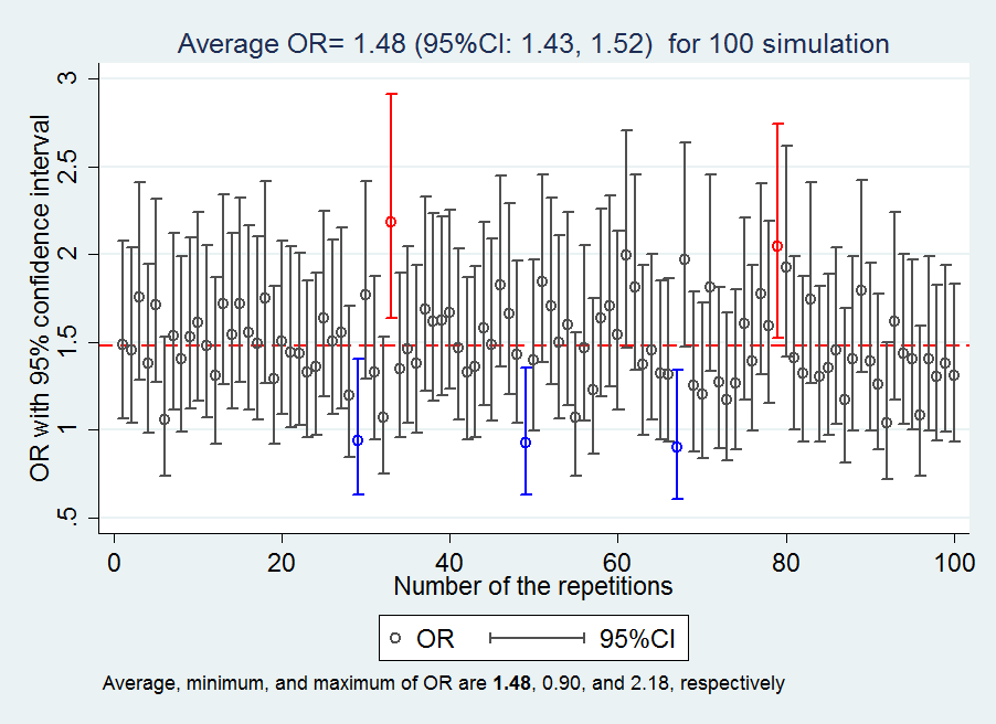
Multiple Simulations and quantification
-
Answers to the questions:
Example 3: Collider stratification bias

-
Interpretation of the DAG:
Under development
-
Curious questions:
Q1: Given the DAG, what the association between the variable E and D would be if the variables I and C are not adjusted for?
Q2: Given the DAG, what the association between the variable E and D would be if the variable I is adjusted for?
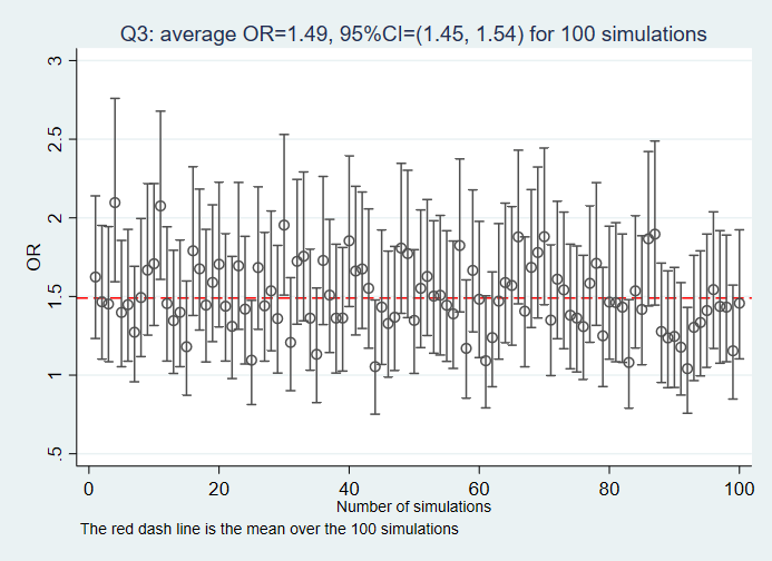
Q3: Given the DAG, what the association between the variable E and D would be if the variable I and C are adjusted for?
-
Simulation and quantification:
Single Simulation and quantification
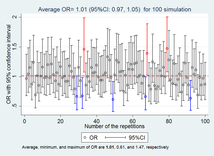
Multiple Simulations and quantification
-
Answers to the questions:
Example 4: M structure or M bias

-
Interpretation of the DAG:
The DAG is so-called M bias (M structure) because the shape of the DAG looks like the capital letter M. M structure is very important because it may revolutionize the definition of the confounder. Traditionally, according to the modern epidemiology (the second edition by Kenneth J. Rothman, Timothy L. Lash,, Sander Greenland), a variable being a confounder has to meet the three criteria:
- A confounder must be associated with the exposure under study in the source population.
- A confounder must be a “risk factor” for the outcome (i.e., it must predict who will develop disease), though it need not actually cause the outcome.
- The confounding factor must not be affected by the exposure or the outcome.
- M is associated with E due to sharing the common cause U1
- M is associated with O due to sharing the common cause U2
- M is not an intermediate variable between E and O (M is not affected by the E or O)
Based on the traditional criteria, if we are interested in the causal association between E and O, we should adjust for the variable M.
On the contrary, based on the D-separate rules, M is a collider variable between E and O and the path (E ← U1 → M ← U2 → O) is blocked. Based on the back-door criteria, if we are interested in the causal association between E and O, we should Not adjust for the variable M. In case, we would have adjusted for M, we opened the path (E ← U1 → [M] ← U2 → O) that was blocked in the first place. Therefore, the adjustment for the collider M leads to over-adjustment and introduce bias, which is called collider stratification bias or collider bias.
-
Curious questions:
Q1: Given the DAG, what the association between the variable E and O would be if the none of the variables is not adjusted for?
Q2: Given the DAG, what the association between the variable E and O would be if the variable M is adjusted for?
Q3: Given the DAG, what the association between the variable E and O would be if the variable M and U1 are adjusted for?
Q4: Given the DAG, what the association between the variable E and O would be if the variable M and U2 are adjusted for?
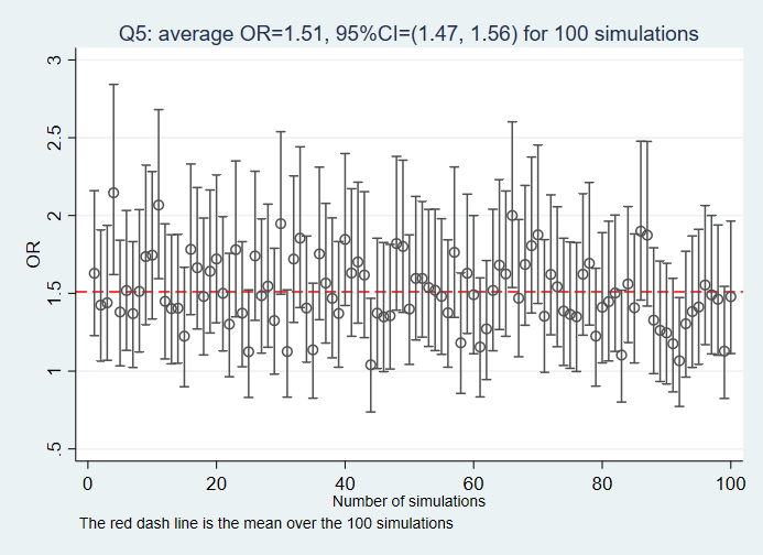
Q5: Given the DAG, what the association between the variable E and O would be if the variable M, U1, and U2 are adjusted for?
-
Simulation and quantification:
Single Simulation and quantification
We are working on this ......
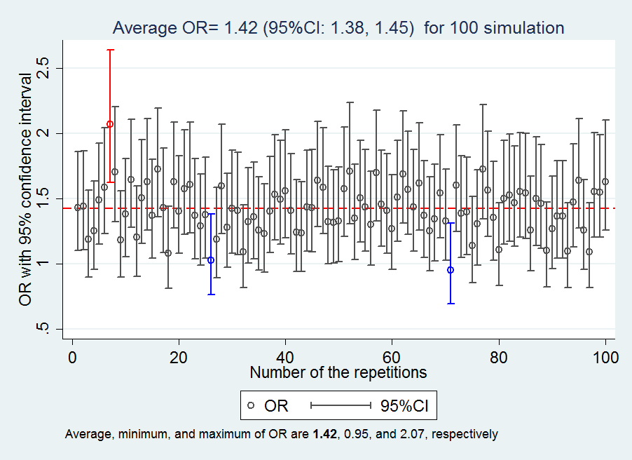
Multiple Simulations and quantification
We are working on this ......
-
Answers to the questions:
Reference
- Greenland S, Pearl J, Robins JM. Causal diagrams for epidemiologic research Epidemiology. 1999 Jan;10(1):37-48
- Hernán MA1, Hernández-Díaz S, Werler MM, Mitchell AA Causal knowledge as a prerequisite for confounding evaluation: an application to birth defects epidemiology Am J Epidemiol. 2002 Jan 15;155(2):176-84
A list of examples of DAG applied to researches
The articles are ordered according to publication date. Please note that MS&DS does NOT necessarily endorse any of the articles. We would like to gradually collect as much as articles we could. If you would like articles to be added, please drop an email to feedBack@medical-statistics.dk.
- Figueiredo ACC et al. Association between vitamin D status during pregnancy and total gestational weight gain and postpartum weight retention: a prospective cohort. Eur J Clin Nutr. 2019 Jul 15.
- Al-Haddad BJS et al. Long-term Risk of Neuropsychiatric Disease After Exposure to Infection In Utero JAMA Psychiatry. 2019 Jun 1;76(6):594-602
- van den Broek S, et al. Thyroid hormone replacement therapy in pregnancy and motor function, communication skills, and behavior of preschool children: The Norwegian Mother, Father, and Child Cohort Study Pharmacoepidemiol Drug Saf. 2021 Jun;30(6):716-726. doi: 10.1002/pds.5184.Epub 2020 Dec 27.
- Anjel Vahratian, et al. Maternal pre-pregnancy overweight and obesity and the risk of cesarean delivery in nulliparous women Ann Epidemiol. 2005 Aug;15(7):467-74. doi: 10.1016/j.annepidem.2005.02.005.
